Shaping Models With BMesh In Blender 2.90
This tutorial introduces Blender’s BMesh as a way to create and edit meshes in Blender through Python. The benefit of BMesh is that we have access to higher level operations than we would working with vertices and face indices; however, we avoid overhead incurred with bpy.ops, the functions called by Blender’s graphical user interface (GUI).
This is aimed at readers who already have already tried their hand at scripting with Blender: who know how to set up Blender to be code friendly, who know how to look up an unfamiliar function in the documentation (either for Python or for Blender), and who know some bread and butter concepts of creative coding.
A prior article on creative coding introduced some of these skills, but has grown long in the tooth. It was written for Blender version 2.79, before significant changes were introduced in 2.8. Other possible starting points include Blender’s Youtube channel
and Diego Gangl’s tutorials, which create meshes from low-level data.
This tutorial was written with Blender 2.90 alpha.
Preparatory Work
Because this tutorial covers the manipulation of vertices, edges and faces, it will be helpful to display the indices of a mesh’s components as a diagnostic measure. To do so, first go to Edit > Preferences…. In the Interface section, under the Display header, tick the Developer Extras checkbox to enable it.

Then, create a mesh object of any kind, and switch to Edit Mode. Open the Viewport Overlays menu and scroll down to the Developer header. Under that header, tick the Indices checkbox to enable it.

Which indices are displayed will depend on context. In the image above, with Vertex select enabled, vertex coordinates are shown for only the selected vertices; in the image below, Edge select is enabled, and so the indices displayed change accordingly.

The font color for the display defaults to blue. To change it, return to Preferences, go to the Themes section, expand the 3D Viewport header, then change the Face Angle Text color.

While beneficial for simple meshes, don’t forget to turn off the display for meshes with high polygon count.
Mesh Creation
Blender offers a few paths to creating a BMesh: from a primitive, from mesh data, from a blank slate and from edit mesh. This tutorial will not address the last due to complications that arise from managing the Blender editor’s state.
Regardless of the source, these examples illustrate the basic template followed in this tutorial:
- Create a
BMesh. - Change the mesh with
BMeshoperations. - Convert the
BMeshto mesh data. - “Free” the
BMeshobject. - Create an object that references the mesh data.
- Link the object to a collection (typically the scene default).
While step 2 will increase in complexity as we progress, the rest will remain more or less the same.
Primitives

To start, remember that Python allows us to import modules under an alias of our choosing; our most fundamental module to import is Blender’s bpy. From bpy, we need data and context; the convention established in Blender's Python Console, is to abbreviate bpy.data to D and bpy.context to C (a capitalized ‘C’).
Our primary concern is with the bmesh module. It is contains four sub-modules: ops, types, utilities and geometry. The lion’s share of creation and transformation functions are in ops, while types will inform us about the structure of a BMesh instance.
Many primitive creation functions require a Matrix from Blender's mathutils module. For the default, Matrix.Identity(4) will suffice. The mathutils module follows the convention of capitalizing static methods to distinguish them from instance methods; hence Identity and not identity.
The function signatures of bmesh.ops methods follow the convention of accepting the first argument, bm, as a positional argument without a named parameter. Subsequent arguments, many of which are optional, should be preceded by the name of the parameter to which they correspond. For example, bm, calc_uvs=True.
Take care when naming objects and mesh data; had another mesh named “Icosphere” been present in memory, a “.001” would have been affixed to the name we supplied to create “Icosphere.001.” As a rule of thumb, avoid retrieving and referencing objects by name. However, there will be exceptions where Blender insists that one chunk of data refer to another by name.

To transform the mesh data (not the object which references it), an affine transform matrix can be created piecemeal, then composited together. The following example creates a cube altered by a matrix.
Use the Diagonal method with a four-dimensional vector when making a non-uniform scalar. Otherwise the method will assume a 3x3 matrix is desired, and then an error will result from the attempt to composite matrices of different dimensions.
Wrap arguments supplied to mathutils entities in a collection: e.g., a tuple, Vector((1.0, 2.0, 3.0)), a list, Vector([1.0, 2.0, 3.0]), or a numpy array, Vector(numpy.array([1.0, 2.0, 3.0], dtype=numpy.float32)).
For those who prefer quaternions, they can be converted to a 3x3 matrix with the to_matrix method. Then, a 4x4 copy of the matrix can be retrieved with to_4x4; alternatively, the matrix can be expanded in-place with resize_4x4. There are also Euler angles, but it is better to get accustomed to matrices and quaternions instead. This is because Euler angles lead to gimbal lock.
Matrix-matrix multiplication is represented by the matmul operator, or the @ symbol. Using a different order of composition than Translation, Rotation, Scale (TRS) as above may give different results.
Other primitives provided by bmesh.ops are: circle, cone, grid, Suzanne and UV sphere. Suzanne is the nickname for what ops refers to as a monkey head. The grid primitive is a plane spanning the x and y axes, with a normal pointing forward on the z axis. The plane is subdivided into quadrilaterals according to the number of horizontal and vertical segments provided. The cone function can also be used to make cylinders.
From Mesh Data

We can also create mesh data from an array of vertex coordinates and indices that specify their order in each face, then transfer the result to a BMesh. This is useful when we want to make a primitive not listed above, or when we want to transform vertices before they are organized into BMesh structures. This example creates a hexagon.
If we calculate the face indices, the edge indices are optional. If we want only the wire hexagon, we can pass the edges with an empty faces list. Setting the verbose flag to True in the mesh data’s validate function is valuable when creating elaborate procedural meshes. To read the output, ensure that the system console is open via Window > Toggle System Console.
To incorporate a transformation matrix, the verts list may be updated to contain Vectors instead:

To double check that the @ symbol interprets the multiplication of a matrix and Vector as the application of a transform to a point (as opposed to a direction with magnitude), a translation can be thrown in as well: transform = Matrix.Shear('XZ', 4, (0.375, -0.125)) @ Matrix.Translation(Vector((1.0, 0.0, 0.0))).
A Blank Slate
If we wish to start with a blank BMesh, we can add BMVerts, BMEdges and BMFaces as we go. In the following example, we approximate a circle with a triangle fan polygon. (To be clear, this particular example has little practical use, since the bmesh.ops.create_circle method accomplishes the same task.)

A BMesh instance's three primary collections of elements — verts, edges, faces— are not lists. Rather, they are of the type BMVertSeq, BMEdgeSeq and BMFaceSeq, respectively. These collections can be iterated over with code such as for vert in bm.verts, but cannot be accessed via subscript without first calling the method ensure_lookup_table. This will be illustrated in the next example. Furthermore, elements within these sequences have a field index that tracks their place. These indices are not updated automatically, so index_update is used.

To transform these elements we use translate, rotate and scale. An advantage of this approach is that we can specify which mesh elements we wish to transform. In the example, a cube’s top face (#5) is translated, scaled then rotated.
In cases where the same verts are targeted by a group of methods, as above, we also have the option of creating a single Matrix, then supplying it to the transform method.
To ensure that verts is a list with subscript access to elements, the slice syntax is used: [:]. The default arguments for this syntax slice from the first to the last element, in effect copying the Blender sequence. The Python list method could also be used.
Supplementary Mesh Data
A cursory glance at the in the Object Data tab of the Properties Editor for a mesh indicates the supplementary information a mesh might hold. The bmesh module can store UV maps and vertex colors. In addition, each sequence of mesh geometry in a bmesh has a layers field which accesses additional information. For example, an edge’s bevel weight may be used to control the behavior of the bevel modifier.
Texture (UV) Coordinates
Suppose we want to use the 2D icosahedral net below instead of the default texture coordinate map.

We extend the from_py_data approach introduced above to add texture, or UV, coordinates to a mesh. This allows us to match the object coordinates and texture coordinates with finer control.
In 3D, the top and bottom rows of faces each converge toward a point at a pole. In 2D, the peaks of these faces remain disconnected. There are more UV coordinates than there are 3D coordinates; however, the number of index tuples and the number of indices per tuple match.
Before the UVs can be added, the verify method is called to ensure that a layer of UV data exists. If it doesn’t, a new one will be created. This method returns the index through which the UV data can be accessed.
Vertex Colors

A similar process follows for vertex color. Instead of using verify, we use loops.layers.color.new. This clarifies that we can make multiple vertex color layers with different names.
Take heed: sometimes Blender requires colors of length 3, with no alpha (transparency), and sometimes it requires colors of length 4, including alpha. While not addressed below, be conscientious of Color Management when working with color by code; depending on Blender’s settings, colors may require gamma adjustment.
The slippage between the terms ‘vertex’ and ‘coordinate’ may be the source of confusion, particularly when building from_py_data. Ultimately, a vertex is not merely a coordinate in space. Rather, it is a collection of data, of which the coordinate is one. However, because a point is the minimal information needed to insert a new vertex into a mesh, and because the point is the most relevant when transforming elements of a mesh, the two are easily conflated. That is why the co needs to be accessed from the vert in the above, but a new vertex can be created with just a tuple.
One way to make generated colors accessible through the interface after the code has run would be to create a color palette through bpy.data.palettes.new. While in Vertex Paint mode, The palette can then be accessed through the Sidebar (keyboard shortcut N), in the Tools tab, under Brush Settings. We could refine this further by preventing duplicate colors from being entered into the palette. Alternatively, we could build a palette (or color gradient) first, then assign them to vertex colors.
In newer versions of Blender, vertex colors can be supplied to a material via the Vertex Color node in the shader editor. (Older versions of Blender used the Attribute node.)
Shape Keys
Blender’s documentation suggests that shape keys can be accessed through bmesh. However, it provides little detail beyond where to access the data, bm.verts.layers.shape. Nor is it clear what the benefit of creating shape keys through BMesh would be. BMeshes roughly parallel the information in mesh data, but shape keys are added to and retained by an object with mesh data. Shape keys associate with a vertex group, again contained by an object. When a vertex belongs to the vertex group used by a relative shape key, the weight provided to that vertex will dictate how much influence a key has.


The images above depict an icosphere with a “Deformed” shape key that warps the original vertices with Perlin noise. The left image shows the mesh in edit mode; the right, in object mode. The color-coding for vertex weights can be viewed in edit mode via the same menu used to turn mesh index display on and off.
Because the vertex weights in “NoiseGroup” approach 0.0 toward the bottom (negative z axis) of the icosphere (colored in blue) while the weights on the top (positive z axis) of the icosphere approach 1.0 (colored in red), and because the shape key is relative, the deformation is more extreme at the sphere's top than its bottom. We've touched on vertex groups before in other contexts, such as visualizing complex numbers and scripting curves. Many modifiers allow a group to regulate the modifier's influence over the mesh.
Examples around the web suggest using the from_edit_mesh and update_edit_mesh workflow. As explained before, this tutorial avoids it. The code below does not use bmesh in any substantive way.
More features of each shape key can be modified than the code above suggests. For example, when a shape key is not marked as relative, different interpolation modes can be specified for its evaluation.
The zip function is a convenience available in Python. The two collections above, data_verts and deformed_sk.data, are expected to be of equal length. By zipping them together, we can iterate through them with an enhanced for-loop as though they were one collection. When constructing the for loop, each element is designated as a comma-separated entry of a tuple.
The noise module contains several flavors of smooth noise. Some methods return a scalar (a float), others return a Vector. The documentation is not always clear what the expected range of the return value is, so experiment with a print line to the console first. Typically, ranges are either in [0.0, 1.0] or [-1.0, 1.0]. Shape keys provide a great way to experiment with layering noise to create terrain. Each noise could be applied to a separate shape key; in the editor, the value of each shape key can be adjusted to change its contribution.
Readers interested in this technique for planetoid generation are encouraged to research what kind of sphere to use as a base. Tutorials may use a icosphere, a cuboid sphere or a Fibonacci sphere, among others.
Custom Primitives
We’re now prepared to create our own primitives, should we find them unavailable in the listed primitives. Before struggling with vertex ordering and face indices, remember that there are many add-ons which expand the repertoire of meshes you can create.
Torus
A torus primitive is available via Blender’s GUI, but is not in bmesh.ops. The maths required to make our own can be found on Wikipedia.

When researching torus mesh code on the Internet, beware. For some graphics engines, it may be preferable to create a torus with a seam. This is particularly so if texture (UV) coordinates are also calculated. The seam results from duplicate, unconnected rings of vertices where the starting and ending azimuth (longitude, meridian) are equal at 0 degrees and 360 degrees; the corresponding UV coordinates at 0.0 and 1.0 are perceptually equal but numerically different. Were the seam not there, the texture would smear from 1.0 - n to 0.0 in the final sector, where n is the amount in unit space covered by each sector.
In the image above, the torus has 32 major segments, or sectors, and 16 minor segments, or panels; 32 x 16 totals to 512 faces. Its minor radius, or thickness, is one fourth the size of its major radius.
The code below is issued in one long block so that it can be copied and run easily. That can make it difficult to analyze, so we preface with an outline:
- Validate user inputs.
- Calculate theta, the angles associated with each sector.
- Calculate phi, the angles associated with each panel, or cross-section.
- Combine theta and phi and the input radii to create the torus’s vertices.
- Construct faces from indices that reference elements in the vertex list.
- Transfer the data to the
BMeshAPI. - If texture coordinates are requested, repeat steps 2–5 for UVs.
- Translate and rotate the
BMesh.
The code above is not written for performance. It is written for clarity. Furthermore, avoiding Pythonic idiom makes it easier to translate to other programming languages. Lastly, it separates code specific to Blender’s API from generic Python. This way, it should be easy to adapt to rely on from_py_data if preferred.
Some may wish the torus doughnut hole to open onto the z axis, as the default Blender torus does; the code above opens onto the y axis. The default quaternion (0.707107, -0.707107, 0.0, 0.0) rotates it by -90 degrees around the x axis.
Although both the list of vertices and the list of face indices are one-dimensional, the vertices were created according to the logic of a 2D grid. For a given corner at (sector j, panel i), there are three more at (j + 1, i), (j + 1, i + 1) and (j, i + 1). These four vertices form either a quadrilateral or two triangles.
At the last sector, we need to wrap around to the first sector at index zero. The same holds for the last panel. This is why we use the floor modulo operator, %, for the vertices. As explained earlier, this is not needed for UV coordinates.
The four corner indices are converted to a one-dimensional index, so we use the formula index k = i * inner_len + j. (This formula may be more familiar in the context of updating an image's pixel array with nested for loops that traverse the image's height and width.)
Mutations
Many analogs to Blender’s modifiers can be found in the bmesh.ops module, including solidify and wireframe. We won't be covering all of them here, but will highlight a few. The documentation already includes one example which creates chain links with spin.
Extrude
Time lapse videos such as 1D_Inc’s demonstrate the power of modeling by extrusion: from point to edge to face an elaborate model can be built. So extrude_vert_indiv looks like a good place to start.

We’ll use a much more rudimentary approach and take a point on a semi-random walk with noise.
Methods in bmesh.ops often return dictionaries that contain the results of the operation. In this case, ext contains two entries. One is a list accessed with the key "verts"; another is a list accessed with the key "edges".
Extrusion is counter-intuitive in that it does not translate the new geometry. The above example deals only with a single vertex at a time, so we can handle the vertex coordinate with Vector operations. After we shift to working with edges and faces, bmesh.ops.translate and other affine transformations may be easier to use.
Note that solidifying this poly-line into a tube is not as trivial as one might hope. Neither wireframe nor solidify are helpful in this regard. As Nikolai Janakiev discusses here, an understanding of Frenet-Serret and parallel transport frames is needed to build a mesh around a poly-line without torsion. Another approach may be working with curve geometry instead.
Moving on, suppose we create a square by creating an edge from a vertex, then by extruding the edge with extrude_edge_only.

This trivial example demonstrates the importance of building skills and understanding by increments, and of turning on diagnostic information. Take a look at this 2D mesh and see if the problem is evident.
When the dictionary returned by an ops method contains "geom", which may contain edges, vertices and/or faces, we have to filter the list with isinstance to find the type of geometry we want.
Were we to extrude the four edges of the square in two dimensions, this would not be a good starting point due to the vertex winding. The new edge created by the extrusion travels in the same direction as the original edge, from left to right (0 to 1 for the original, 2 to 3 for the extruded copy).
We could get around this by sorting our 2D vertices. For example, the key parameter would accept a function that returns the heading, or azimuth, of the vertex coordinate: math.atan2(v.co.y, v.co.x). More in-depth discussions on sorting vertices can be found here and here.
A better starting point would be a polygon, whether it be created from_py_data or from a primitive.

In the following example, create_circle is used to make a pentagon with a central point and triangle fan faces. If preferred, we can create an n-gon by changing the argument given to the parameter cap_tris to False.
An important check performed in this code is whether an edge is an interior edge or a boundary edge. As labeled in the image above, edges 0, 3, 5, 7 and 9 are boundary edges; edges 1, 2, 4, 6 and 8 are interior edges. We don’t want to extrude the two edges emanating from the center point of the pentagon which join triangles in the fan.
The vector cross product is used to find a a direction perpendicular, or orthogonal, to the input vectors.
In this case, we use the face’s normal and the edge’s vector. We find the edge’s vector by subtracting its destination point from its origin point.
The terminology here can be confusing. A vector is usually explained within the framework of physics as a direction with a magnitude (or length). The direction is described in Cartesian coordinates. However, in computer graphics, a vector means just about any doublet or triplet of real numbers designated by x, y and z. Depending on implementation, this may include vectors (in the former sense), points, colors and normals.
Once we have a vector, we separate it into magnitude (through the Pythagorean theorem, or sqrt(dot(v,v))) and a direction (through normalization). This is why vertex winding was an issue in the extrude_edge_only code above. If a two-dimensional edge has unconventional vertex winding, the direction from origin to destination will be reversed. The orthogonal vector returned from the cross product would point inward, not outward.

Lastly, we can extrude faces with extrude_discrete_faces. Above is an icosahedron whose faces have been extruded along their normals.
In addition to extruding faces individually, we could also use extrude_face_region. This alternative returns more general information, "geom", which would need to be filtered, where as the discrete version above returns faces. Furthermore, the original faces would need to be deleted with either bmesh.ops.delete or a BMesh instance's faces.remove.
In Vectors, the matmul operator, a @ b, is a shortcut for the dot product, a.dot(b). The dot product is the sum of the product of each vector's corresponding elements: in 3D, a.x * b.x + a.y * b.y + a.z * b.z.
Inset

Insetting a face with code is similar to doing so via Blender’s GUI. When insetting via the interface, the I key toggles between individual and regional inset. This is equivalent to choosing between the BMesh methods inset_region and inset_individual. The finer points of these two methods remain undocumented, so consulting the manual is recommended.
A step pyramid, pictured above, is the obvious exercise to try our hand. The individual inset is used to create the flanks of the pyramid; the regional inset is used to add some detail to the horizontal steps.
Python does not have an strict analog to the ternary operator used by languages with C-like syntax, where a = condition ? b : c translates roughly to "assign b to a if condition is the case; else, assign c." However, a one-line if-else expression can be used, a = b if condition else c.
Mirror, Symmetrize
As proposed by Greg Lynn, symmetrical form can be thought of as a loss of information:
[William Bateson] was what you’d call a teratologist: he looked at all of the monstrosities and mutations to find rules and laws, rather than looking at the norms. So, instead of trying to find the ideal type or the ideal average, he’d always look for the exception. So, in this example, which is an example of what’s called Bateson’s Rule, he has two kinds of mutations of a human thumb. […] [I]nstead of having a thumb, you would either get another opposable thumb, or you would get four fingers. So, the mutations reverted to symmetry. And Bateson invented the concept of symmetry breaking, which is that wherever you lose information in a system, you revert back to symmetry. So, symmetry wasn’t the sign of order and organization — which is what I was always understanding, and as is an architect — symmetry was the absence of information.
Mirroring organic models is a handy way to create chimeras and monstrosities. In the example below, we remix models from Scan The World, in this case the Seated Virgin Mary, for illustration.

The model is mirrored with a transform matrix, adding greater flexibility than the ortho-normal axes x, y and z initially permit.
The symmetrize function is similar. The directions supplied to the function can be signed, e.g., '-Y' and 'Y', for greater control over which side of the axis to mirror.
Convex Hull
When discussing shape keys above, we mentioned the importance of choosing a sphere in the creation of a rough planetoid through noise. One option was to distribute points on the sphere’s surface according to the golden ratio, then form edges and faces around those points.

More sophisticated treatments on this subject are available via Red Blob Games. For our purposes, a situation in which we have a set of points that we do not know how to connect lends well itself well to using a convex hull.
The dictionary returned by the convex hull method contains four entries: "geom", "geom_interior", "geom_unused" and "geom_holes".

The convex hull operation under the Mesh menu in edit mode is a handy way to preview what the bmesh version will do to a given mesh.
Unsubdivide & Split Edges
The unsubdivide method matches an option in the decimate modifier. It is popular for creating diamond patterns on meshes such as a UV sphere.

In conjunction with split_edges, it can be used to add detail to surfaces.

We match the individual origins pivot point by finding a center of a face and treating it as the pivot. We translate by the negative pivot prior to rotation or scaling, then add it again after.

To consolidate these two, the example below creates an spiral, which is then broken up into diamond faces. The diamonds are then extruded from 2D to 3D. A bevel is added for detail.
When extruding an edge, finding the perpendicular is a shortcut for the cross product method used earlier. Depending on which perpendicular we want, we use either perp(a) := (-a.y, a.x) or perp(a) := (a.y, -a.x).
For bevel, the 'PERCENT' offset type renders the input value as it would be displayed in a GUI, e.g., 5% is 5.0, not 0.05. The method signature is different between version 2.83 and 2.90 alpha of Blender, so the code may need to be changed to use the vertex_only parameter rather than the affect parameter. The vertex_only flag accepts either True or False. The affect parameter accepts either 'EDGES' or 'VERTICES'. Blender's version can be accessed in code via bpy.app.version, which returns a tuple with three elements.
Planar Bisection

We end with planar bisection because its creative potential is easy to see. There is no direct analog to it in the GUI’s list of modifiers; rather this operator corresponds to the bisect found under the Mesh menu in edit mode.
Imagine a plane of infinite extent; such a plane can be represented with two arguments: a coordinate and a normal. The normal represents a direction orthogonal, or perpendicular, to the plane’s surface. If such a plane were to intersect with a mesh, we could specify a portion of the mesh that fell beneath the plane and another portion that fell above the plane.
When a mesh is cut by a plane, no new geometry is added to the mesh along the cut. The resulting meshes can wind up looking hollow. One way to deal with this is to use edgenet_fill to create a new face. The result works best when topology and smooth normals are not at issue.
The question is how to get the edges created by the cut. We reference the documentation to find the relevant dictionary key, in this case the string (str) "geom_cut". The value retrieved by this key is a list that needs filtering.
The reverse operation is also necessary: lists of mesh data with different data types may need to be concatenated into one list. Because Python relies on a line break, not a semicolon, to terminate a command, the backward slash, \, is used to break up the concatenation above without causing a problem.
For the second slice, The Boolean flags supplied to the clear_inner and clear_outerparameter have been flipped.

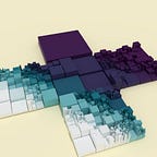
Another illustration of planar bisection draws inspiration from a scene in The Cell (2000) directed by Tarsem Singh. The scene pays homage to Some Comfort Gained from the Acceptance of the Inherent Lies in Everything (1996), attributed to Damien Hirst.
We section a source mesh into separate, animated objects. To do this, we first create a function similar to that found under Object > Set Origin > Geometry To Origin. This serves two purposes. First, it allows us to distribute the number of cuts we want to make evenly. Second, for the benefit of animation, each newly created mesh has a central pivot.
Once we know the lower and upper bounds of an imaginary axis-aligned bounding box (AABB) that surrounds a given mesh, we can shift the vertices of the mesh’s data. We can then then change the location of the object that holds the data. Another function we need is a vector easing function to distribute each slicing plane evenly between the lower and upper bounds. Linear interpolation is below.
Instead of creating a new face along each cut, as with the cube above, each new mesh is solidified. The Suzanne model is less than ideal for either approach, but useful to illustrate some of the pitfalls when choosing a source mesh to slice: Suzanne’s eyes are disconnected from the rest of the mesh. Also, some of the creases which connect the ears to the skull are sharp. The latter can result in spikes if a solidified mesh’s thickness is too great.
Before the mesh is split, it is subdivided to add some more polygons. The subdivision surface modifier does not correspond one-to-one to the subdivide_edges method, at least not in terms of input parameters, so tinkering may be needed to get desirable results.
Instead of cutting with a random plane, the above code proceeds from left to right on the x axis. A bias is added, -0.5 and 0.5, ensure the cuts fall before and after the center of the segment.
Once the slices have been converted to objects, we then animate them by inserting keyframes. The property to be animated is supplied to the insertion function as a String. To reduce clutter in the Outliner, slices are parented to an empty object. The first and last frame of the scene's timeline are set to matching keyframes, while the middle frame gets a keyframe for a new location and rotation. As a reminder, the // operator indicates integer division.

It is also possible to section a mesh like an orange by generating plane normals with a spherical to Cartesian conversion. The plane coordinate remains constant across each iteration, at a center of the mesh. The azimuth would increase per slice. The example above uses the model Bust of a Bearded Old Man, with an alternating material to accentuate the slices.