Scripting A Hexagon Grid Add-On For Blender 2.91

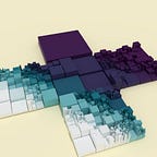
This tutorial explores how to make a grid of regular convex hexagons in Blender with Python, then how to turn that script into an add-on. An example render made with the add-on looks like so:

The tutorial takes inspiration from the hexagonal basalt columns of the Giant’s Causeway in Northern Ireland and Fingal’s Cave in Scotland. Such formations have also inspired the environs in video games such as Dark Souls II, Dragon Age: Inquisition and Skyrim: Dragonborn, to name a few. A caveat: this tutorial does not explain how to create photo-realistic basalt columns with the natural irregularities of those pictured at the top. A Voronoi mesh generator might be more useful for readers with such a goal.
Those wishing to skip to the full code for this tutorial may reference the Github repository.
This tutorial was written with Blender version 2.91. Blender has evolved rapidly over the past two years; please consult the release notes for changes between that version and the current one.
Hexagon Basic Geometry
First, let’s review some geometry. Suppose we position the hexagon in a Cartesian coordinate system at the origin, (0.0, 0.0), where the positive x axis, (1.0, 0.0, 0.0), constitutes zero degrees of rotation. Positive on the y axis is forward, (0.0, 1.0, 0.0), and positive on the z axis is up, (0.0, 0.0, 1.0), which means that increasing the angle of rotation will give us counter-clockwise (CCW) rotation.
We follow the convention of Blender’s 2D mesh circle primitive, where the initial vertex starts at 12 o’clock, not at 3 o’clock. In consequence, the hexagon is standing upright, not flat on its side.
Since a regular convex polygon is a constant shape, we can hard-code its features to avoid converting from polar coordinates to Cartesian coordinates via sine and cosine. In the table below, we assume that the first vertex is at the center of the hexagon.

The key numbers here are the square-root of three, 1.7320508, and its division by two, 0.8660254. A hexagon’s radius multiplied by 0.8660254 is the distance from the hexagon’s center to an edge’s midpoint. If we tile hexagons leaving no gaps between, then to travel from one hexagon center to another across an edge we would travel two such lengths, 1.7320508.
This is explained in greater detail in the Parameters section of the Wikipedia entry on hexagons. The circumradius, or maximal radius, R (green) is the distance from the center to a vertex. The inradius, or minimal radius, r (blue) is the distance from the center to an edge’s midpoint.
For the sake of topology, we may also want to subdivide the hexagon. The subdivisions available depend on whether we want to insert a vertex coordinate at the hexagon’s center and/or bisect edges of the hexagon to create new vertices at edge midpoints.

In some cases, the need to ensure that a hex grid is composed only of triangles before the model is exported will drive our decision. In other cases, we may be interested in the pattern generated by the subdivision after tessellation.

For example, subdividing a hexagon into three quadrilaterals creates — along with color choice — the optical illusion of stacked cubes in an isometric projection. More possibilities are illustrated in the Wikipedia article on hexagonal tiling, here.
Echoing The Manual Approach
Next, we consider how we’d create a hexagon grid manually, with Blender’s graphical user interface (GUI). Afterward, we’ll recreate that algorithm in Python script. zerobio provides a tutorial on how to do this:
In the first leg of the process, we create a circle primitive with 6 vertices, append an array modifier for the horizontal offset, then append an array modifier for the vertical offset. For those unfamiliar with the BMesh workflow, a prior tutorial offers an introduction.
As far as parameter names for create_circle go, cap_ends fills the shape with a ngon when True; cap_tris fills with a triangle fan instead of an ngon. Generally, the first argument in a bmesh.ops method, bm, is positional; all subsequent arguments, such as segments and radius, should be supplied with the parameter named. Many of the named parameters listed in the API can be assumed to have default arguments.
For the ArrayModifiers, zerobio uses relative offsets. Either relative or constant offsets will work, given appropriate measurements. For the second array modifier that creates the grid’s rows, the relative horizontal offset is 0.05 because half the mesh’s width, 0.5, is divided by the count used in the first (horizontal) array modifier, 10.

The advantage of this approach is that it uses out-of-the-box methods, making it fast and easy; it’s also non-destructive insofar as it uses modifiers.
The main disadvantage, which zerobio shows how to fix, is that the grid forms a parallelogram. To make a rectilinear grid, the array modifiers need to be applied (removing an aforementioned advantage). Sections of the parallelogram then need to be snipped and rearranged. Another minor inconvenience is that the grid’s origin lies in near the bottom-left corner, in the original shape’s center. The grid could be centered with Object > Set Origin > Geometry To Origin, but it’d be nice if it were centered right away.
Were we to pursue this route further, we could try to square the parallelogram with code, perhaps with a series of orthonormal planar bisections, or with a boolean intersection between the hex grid and a cuboid.
Hexagons in Concentric Rings

Instead of the modifier approach above, we’ll aim to create an add-on which appends a grid of hexagons to a collection from the Add > Mesh menu of the 3D viewport when in Object mode. We could create a staggered square grid instead, but given that our inspiration is natural, not artificial, arranging our hexagons in concentric rings is a better fit.
Many inputs in the screen capture above should be self explanatory. The terrain type is an enumeration that specifies a shaping function for the extrusion of the grid on the z axis. This tutorial addresses four shaping functions: uniform, linear gradient, spherical gradient and conic gradient. These are the same functions we used to make color gradients in Processing. Any function that accepts an origin and destination point as inputs and returns a factor in [0.0, 1.0] will work.
This terrain factor is mixed with a noise factor according to a noise influence. The result is used to interpolate from the extrusion lower bound to the upper. The remaining 3 inputs will be supplied to one of Blender’s noise methods.
We’ll start with the business logic, then include more data related to Blender’s GUI later. As an exception, one GUI-related item we’ll include right away: a class which will be recognized as an operator. In Python, to extend a class with a sub- or child- class, we specify the parent, bpy.types.Operator, in parentheses after the class name and before the colon.
For ring count, we include the central hexagon as the first ring, then set the minimum number of acceptable rings to one. That way, at least one hexagon will be created. orientation indicates how much to rotate the grid as a whole around the z axis after it is created; in the code above, we haven’t made use of this parameter yet. face_type specifies the manner in which a hexagon is subdivided; we’ll address this in the next code snippet.
In case we need to organize our faces and vertices by hexagon, we’ll create two dimensional lists for verts and faces. For each iteration through the inner loop, a list of hex_vs and hex_faces will be appended.
When finished this method will generate a 2D grid similar to this:

The logic to create this grid is sourced from Red Blob Game’s extensive articles on hexagonal tessellation and coordinate systems. To grasp how these nested for loops work to create the grid, it is helpful to add diagnostic print statements for indices i and j.
For 4 rings, i will span from negative to positive rings-1. The number of hexagons added per iteration of the outer loop will begin with 4 and increase by 1 until we reach the central iteration, where i is 0 and 7 new hexagons are added. Afterward, the hexagons created will decrease by 1. The total number of hexagons created, 37, is equal to 1 + i_max * verif_rings * 3. Depending on face_type, that number will need to be multiplied by faces per hexagon to predict the total number of faces.
To add faces, we introduce the following:
When the BMVertSeq is called to create a new vertex, a BMVert is returned. All we need to supply to the new method is a collection — tuple, list, Vector — that specifies the vertex’s coordinates (conventionally shortened to co in Blender’s API). Even though the mesh is 2D up to now, we should still provide a third component for z, 0.0. To append a new BMFace in the BMesh’s BMFaceSeq, we need a collection of BMVerts.
The code snippet above shows only points, tri fan, quad fan and ngon options; more options are supported in the full Github repository. For face types which require edge midpoints to be calculated, an edge’s origin and destination vertices are added, then the sum is divided by two to find the midpoint.
Once we’ve finished creating faces in the nested for-loops, we merge duplicate vertices if requested. Next, we calculate the width and height of the grid overall. This allows us to rescale coordinates in world space to texture coordinates in [0.0, 1.0]. We create a 4x4 rotation matrix with Matrix.Rotation using the z axis, (0.0, 0.0, 1.0); since a 3x3 matrix is sufficient to hold a rotation, we specify that the desired size is 4. We ensure the mesh’s normals are updated, then return a dictionary with the faces.

Because the grid is wider than it is tall, UV coordinates (left) will be squished horizontally; this results in a square image looking stretched horizontally on the mesh (right). If desired, this can be corrected with the grid’s aspect ratio, width divided by height.
Extrusion
We could stop there if that’s all we needed. However, manually configuring a SolidifyModifier to vary the extrusion with noise or according to a shaping function can take a few steps in the GUI.

For that reason, we’ll make a separate extrude method which accepts the list of faces generated by the prior method. The method will return True if all inputs were valid and the extrusion has occurred; False if not.
We tackle the simplest case first: where there is no margin between hex cells and the user has specified that overlapping vertices be merged together. In this case, we allow only uniform extrusion.
The bmesh.ops.extrude_face_region method accomplishes this task. When the use_keep_orig flag is set to True, the original faces are retained. These will become the bottom faces of the hexagonal prism. This method does not translate the new geometry it creates. The information it returns needs to be filtered. Because bmesh.ops.translate accepts vertices, we append all elements from the extrusion results to a list if they match the type BMVert.
The snippet above could be briefer and clearer were Vector math used. For example, dot_ab could be assigned the result of a.dot(b). However, as a precaution, we treat input arguments as if they were tuples. The elements of a vector can be accessed with either a subscript or the axis. For example, a[0] and a.x should return the same number.
The calculations we need to make depend on the requested shaping function. Linear gradients depend primarily on scalar projection of one vector, a, onto another, b. In this case, a is the difference between the line’s origin and the hexagon’s center; b is the difference between destination and origin. Spherical gradients depend on finding the ratio of hexagon center’s distance from an origin to a maximum distance. Conic gradients depend on finding the azimuth, or heading, of a vector, then converting the angle to a factor.
Once the above factor is found, we introduce some noise (i.e., smooth randomness). The mathutils.noise submodule offers a variety of noise methods, including those meant for terrain; however, because the hexagon grid is of such a low resolution, we chose a simple one.
The consequence of extrusion on the grid’s face indices can be seen below:

If the 2D grid originally contained 37 ngons, then the first hexagonal prism, left center, will have face 0 as its bottom and face 37 as its top. Each subsequent top face will be an increment of 7 from the previous (37, 44, 51, and so on). The quadrilaterals on the sides will use the intermediate indices, though not in a clockwise or counter-clockwise order. In the case of the first prism, we see indices 38, 40, 43, 39, 42, 41 CCW from the 12 o’clock vertex. We have the option to sort vertex and face sequences if we wish.
The grid’s UV texturing is also impacted. The side panels will look streaked:

The extrusion copies the bottom face’s UVs to the top. This tutorial will leave this as is. Those who wish to change it via script will find that newly extruded faces can be found via the filtration-by-type approach used above. The UVs can also be adjusted manually by entering Edit mode, selecting a side face, going to Select > Select Similar , then selecting an option from UV.
Coding The Add-On
Last, we turn to the code which will provide a user-friendly interface for the business logic created above. Much of what is covered here can also be learned from the manual or the video series Scripting for Artists.
First, we’ll add the information to display when the add-on is searched in the Edit > Preferences > Add-ons menu.

This is done by adding a dictionary called bl_info after the imports and before the class declaration:
"version" signals the current version of the add-on; it can be an indirect way of communicating to the user how developed the add-on is. For example, version (1, 0) or 1.0 would be the add-on’s initial release to the public, whereas (0, 13) or 0.13 would signal that the add-on is still early in development. Guidelines on semantic versioning, such as this one, may help with the decision of when to change the add-on version.
The "blender" field indicates the version of Blender the add-on is intended to work on. To find the current version of Blender in use via Python, check bpy.app.version.
We next add some apparatus related to registering and unregistering our add-on. The register and unregister methods are called when we tick the checkbox next to an add-on in the Preferences menu to enable and disable it.
The poll method indicates the proper panel wherein the add-on will operate; this conditions when the add-on appears in a search. To help select which icon we associate with the add-on, we can enable the Icon Viewer add-on in preferences, select the icon visually, then copy the string used to identify the icon.

Next, we add properties to the HexGridMaker class. These properties will dictate what inputs appear in the redo/undo menu, the tooltips that will appear on mouse hover, and the upper and lower bounds that govern valid input ranges.
Properties are assigned with a colon, :, not an equals sign, =. Using the latter will print a warning in the terminal. The snippet below doesn’t show all the necessary inputs for a hex grid, just enough for illustration.
Numeric properties contain a min, max pair and a soft_min, soft_max pair. The soft bounds limit the value when the mouse is passed horizontally over the field; the hard bounds also limit keyboard input.
Real numbers, i.e., FloatPropertys, include step and precision. step specifies as a percent how much to increment and decrement a value when the < > buttons on the end of a input field are pressed; this takes an integer value which is divided by 100. precision specifies how many places right of the decimal to display. Generally speaking, for small values, the defaults are not fine enough and need to be increased.
For FloatVectorPropertys, make sure that the dimensions specified by size matches the default collection’s length; for example, (0.0, 0.0) should match 2; (0.0, 0.0, 0.0) should match 3.
EnumPropertys can get fairly involved because items is a list of tuples. Within each tuple, the first string represents how the enumeration constant is represented in code. The second string represents how the constant is displayed in the GUI.
Lastly, we hook our business logic together in the execute method.
The second input of the execute method is a context; we use that over bpy.context. The main logic here is to create mesh data, unload the BMesh into the mesh data, assign the data to an object, and link the object to a collection in the scene.
Conclusion
There are any number of ways the add-on created in this tutorial could be improved. For example, we could offer more ways to arrange hexagons in a grid; a toggle to create separate objects each with its own hexagon mesh instead of one mesh; greater control over UV coordinates; more shaping functions; more refined control over noise; and so on.
The fine line with add-ons is to create just enough convenience without adding too many features. Feature bloat makes the menu difficult to read and, at extremes, makes the user feel like they need to read documentation just to understand how the add-on is used.