3D Transformations in Processing

This tutorial explores how translation, rotation and scale — taken together under the umbrella term affine transformations — work in Processing (Java mode). An alternative to matrices, based on a quaternion, is then created to show how we can ease between ‘keyframes.’ To keep this tutorial from being any longer than it already is, the code gists to follow contain only highlights under discussion. Full code for the classes and functions can be found here.
This tutorial was written with Processing version 3.3.7 in the Processing IDE (as opposed to Eclipse, etc.). Since coding with multiple objects requires a learning curve, one helpful feature to turn on is code-completion, to be found in the File > Preferences menu.
Pushing Matrices with Native Functions
Order of Operations
Just as mathematical operations have a conventional order (PEMDAS), so do transformations of a shape: translation, rotation, scale (TRS). Until we adjust to this ordering, as Rodger Luo points out in “One Small Trick about Transformation in Processing,” our code may produce unexpected results.
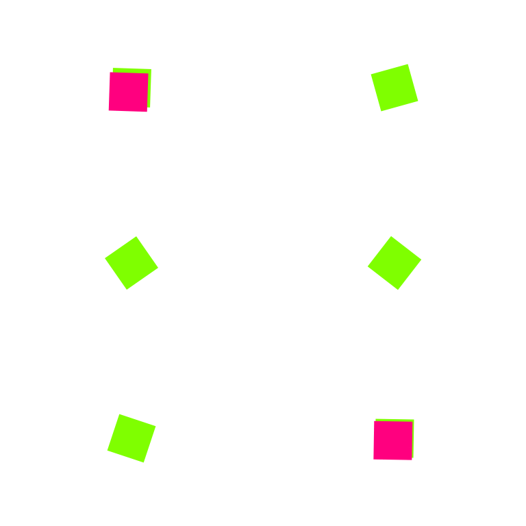
The magenta square orbits around the top-left corner of the sketch, appearing only 25% of the time, while the green square rotates in place at the center. To understand why, we try out six possible orders (TRS, RTS, RST, SRT, SRT, TSR, STR) on the underlying matrix (PMatrix3D for the 3D renderer), then look at the print-out.
Before we look at the results, a sidebar:
Sidebar: Keep Rotations Simple

The test above is a simplification of even the simplest use-case where Euler angles are supplied to rotateX, rotateY and rotateZ. Taking that into consideration would mean another six operation orders (XYZ, XZY, YXZ, YZX, ZXY, ZYX) per each of the six above. Instead, we rotate by an angle around an axis.
The difference between axis-angle and Euler angle rotation is most noticeable with the wobbling magenta cube on the far right. A caveat: the axis should describe only direction, not scale. This means the vector should have a length of one, and therefore lie on the unit sphere. For this reason, it is normalized.
Notation
To return to the first code snippet, by comparing the results of TRS and TSR
with the other four orders, we can guess that translate is influenced by rotate and scale, and so should come first. Before we look at translate’s definition, we reintroduce the matrix notation used from a previous tutorial on rotation, where each cell corresponds to a float in PMatrix3D:
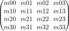
This was supplemented with a more intuitive notation, where the columns represent the right (i), up (j) and forward (k) basis vectors for a spatial coordinate, color-coded in red 0xffff0000 for i; green 0xff00ff00 for j; and blue 0xff0000ff for k. t represents the translation. The rows represent the vector components x, y and z. The row value belongs to the column value.

Were we to represent a matrix with a 2D array instead of as an object,
programming conventions would suggest that columns belong to the rows. This could then be re-envisioned as
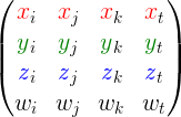
This point is belabored because (1.) to understand transformations we must switch between these two orderings; (2.) transposing a row index with a column index is an easy mistake to make; (3.) PMatrix3D’s loose floats, make it easy to switch between thinking in rows and in columns.
Translation and Scale
With that under our belt, let’s look at the definition for translate in the source code
Scale, by comparison, is straightforward:
Taken all-together with rotation, these operations can be represented as

Width (w), height (h) and depth (d) are the components of non-uniform scalar n. For n, multiplication is defined as v * n = (v.x * n.w, v.y * n.h, v.z * n.d).

What this does not adequately capture from the source code is the += in translation and *= in scale. These operations are cumulative; they do not set the matrix to a particular translation or scale. This accumulation comes into play when we nest one transformation within one another.
Nesting Transformations
To illustrate nested transforms and spatial locality, consider a model of the solar system prior to the advent of Newtonian physics. The sun is at the origin of the solar system; the earth is a child of the sun; the moon, a child of the earth. Humanity’s place within this universe could be solipsistic, geocentric or heliocentric. With Processing’s built-in tools, such a model can be coded as

With each pushMatrix, a matrix is pushed onto a stack data structure. Stacks follow Last-In, First-Out ordering (LIFO), so we create and apply transformations in the order 1–2–3; we remove (popMatrix) them in the order 3–2–1. Should we wish to replicate this process independently, we could take an approach such as
Where applying the matrix inverse reverses the impact of its multiplication, and could be thought of as matrix division. Care should be taken, however, matrix multiplication is not commutative, i.e., m * n != n * m.
Processing calls multiplication of this matrix m by an operand to the right, n, apply. The multiplication of this matrix n by an operand to the left, m, preApply.
Trees / Hierarchies
Conceptually, this ‘solar system’ can be thought of as a tree. Each node can have multiple children, but only one parent. E.g., the sun has eight planets; Jupiter, 69 or more moons. If a node has no parent, it is the root node; if it has no children, it is a leaf node. This leads to a hierarchical structure, where any change to the root node cascades down to its children, grandchildren and all ancestors thereon. The distance of a node from the root is its depth; a maximum depth for the tree can be found by seeking the deepest leaf node.
This hierarchy may expand in either direction, moving up to the Milky Way Galaxy, or down to the limbs of the human body. We visualize it with tabular indents, as in Unity’s hierarchy panel, or with nodes and edges.

Since a goal of this tutorial is to open new possibilities for animation, we note that anthropoid skeletal rigs can be described by such a tree.
Decomposing Transformations
Processing functions model and screen let us cache coordinates relative to a tree node; however, if we want to know the translation, rotation and scale of a matrix, we decompose it. To do so, we refer to this discussion at Stack Overflow and Three.js, keeping in mind that Processing flips the vertical axis from the OpenGL standard. For the P2D renderer, we use
The way getMatrix and these decompose functions work may be unfamiliar. We expect a function like getObject() to return a new instance of that data-type. Creating a new object every frame of animation is expensive, so functions that work with expensive objects accept an ‘out’ parameter. This ‘out’ is an instance of that object that has already been created; the object’s values are set within the function. Additionally, if ‘out’ is not supplied, getMatrix(); doesn’t know whether we want a 2D or 3D matrix, and we have to cast the result,(PMatrix3D)getMatrix();.
Although 3D is our focus, note that Processing’s other 2D rendering modes, JAVA2D and FX2D, rely on the AWT and JavaFX libraries respectively. Readers interested in carrying the concepts across will need to research how those libraries implement a transform matrix.

Back in 3D, the biggest difference is that we have many ways to represent rotation. Here, we use Euler angles. Finding the determinant is required for extracting a matrix’s scale; it’s tidy enough in 2D, but is heftier in 3D.
We take rotation order — XYZ — for granted; to be robust, we’d have to account for all possible orders. We also assume a fixed camera. If it is animated with the camera function, the matrices representing the sketch’s projection, project-model-view, and so on may be worth taking into account. Such matrix data can be accessed by creating a PGraphics3D variable to which (PGraphics3D)g; is assigned after size is called in setup.
A Custom Transform
Transforms that use a quaternion are an alternative to the matrix-based approach above. Before creating our own, we’ll jot down some criteria we’d like to meet.
Writing A WishList
We want our transform to be
- Consistent — two functions with the same name behave the same way.
- Concise — as much code as possible is shifted into
setupand into class methods. The transform is animated in thedrawloop with few lines of code. The transformation of one shape influences only that shape. - Clear — functions are named so we can distinguish between transformations of a shape by a value, to a value, or between values over a step in time. We can debug transforms visually and in the console.
- Capable — transforms can be parented to one another. The position, rotation and scale of a transform in world space can be accessed and mutated (without having to decompose a 4x4 matrix). The right, up and forward axes of a transform can be accessed.
Fair warning: since we’re deviating from Processing’s default tool-set, a lot of setup will be required before we see a payoff.
Transformable Elements
It is common for programming languages to represent a color, coordinate, Euler angles, non-uniform scalar, normal, direction and just about any triplet of real numbers with a vector. An advantage in doing so is that there is less code to write and maintain. Additionally, functions are less picky; we won’t throw an error because we’ve supplied a vector to a function that wants a coordinate. Last, since much joy in creative coding is synaesthetic — representing time as scale or space as color, for example — the borders between senses are easier to cross when one data container is all we need.
A disadvantage arises from its obscurity. When learning vectors, the blackboard explanation bears little resemblance to how they’re used in code. Vector functions are inappropriate to the data stored in x, y and z.
Tutorials and libraries with all-purpose vectors are easy to find, so for variety’s sake we’ll separate these triplets out. There is a hazard to to taking this route, indicated by the Circle-ellipse problem, which will not rear its head immediately; we give it a name now so as to better spot it later. Mattias Petter Johansson has a great discussion about this (targeted at JavaScript) in “Composition over Inheritance.”
Insofar as these various data containers are similar, we want to guarantee that they share behaviors: the ability to compare one against the other and therefore to be sorted; to check for approximate equality between floats; to reset to a default value; to copy another instance of the same type with a set function. We create an interface to code this guarantee. This will also help us maintain consistent function names.
To follow through on this guarantee, we’ll need a reliable way to approximate floats. For this, we refer to The Floating-Point guide. While we’re at it, now’s a good time to cover other needed utility functions, namely floorMod.
The % operator will return a negative value when the right-hand operand b is negative. floorMod returns a positive value. This is handy for setting an Euler angle to a range 0 .. TWO_PI or screen-wrapping a moving object (as in Asteroids). The naming convention for these two functions varies among programming languages; we stick with that of Java’s Math library, which includes floorMod for ints and longs.
Tuple
We start by creating an abstract class as a parent for point-like types with three named floats. For those unfamiliar, a class is commonly analogized as a ‘blueprint’ for instantiating object; an abstract class is not intended for direct instantiation, but for passing on blueprint information to child- or sub-classes.
In the big picture, this approach will consist of pushing upward into abstraction: if we find ourselves writing the same function repeatedly for each class that extends Tuple, then we can move that function into Tuple itself.
Because classes defined within a Processing .pde file need to be static to define a method such as static Tuple sub(Tuple a, Tuple b) { /* … */ return new Tuple(x, y, z); }, we adopt an unconventional format: binary methods like addition and subtraction accept two inputs a and b. The result is assigned to the tuple instance that called the method. For unary methods, such as a vector’s normalize method, the input is named in.
When comparing two Tuples for the purpose of sorting them, the compareTo function mandated by the Comparable interface returns -1 when Tuple a is determined to be less than b, and should precede b in a list sorted in ascending order; when a is greater than b, 1, and should follow b; when the two are equal, 0. The ternary operator is a shorthand for if(a.z > b.z) { return 1; } else { /* … */ }. This means that z is the most important criterion when sorting two Tuples, followed by y and then x.
Next up, a spatial coordinate class:
Coordinate
For now, this class does not need much. Why bother? An example of where the distinction between coordinate and direction comes in handy is the lookAt method. When we want one object to look at another, we can create lookAt(Coord origin, Coord destination, Vector up);. When we want it to look in a direction, we can write lookAt(Coord origin, Vector lookDir, Vector up);. Furthermore, were we to support a matrix class, we could add a w field to Coord to support multiplication between them.
Where possible, the principle of chainability is kept through having math operations return Tuple;, return Coord;, and so on. This can lead to confusion later. Suppose we add two coordinates, Coord c = new Coord().add(new Coord());. This throws an error because the value returned is of the type Tuple. It makes more sense to say that Coord add(Vector v); represents moving from one spatial coordinate to another by a direction. The larger point is that sometimes a designer withholds functionality — even when adding it would make life easier — because it distorts how code models reality. The GDC talk “Understanding Homogeneous Coordinates,” left, is helpful in explaining the addition of points and directions.
Direction
This class is called Direction, not Vector, for a reason. Directions which instruct the computer how to interpret light and shadow on a surface are called normals. These are not necessarily normalized, and not to be confused with the normalize function. Shown the image to follow, Processing computes light and shadow on our behalf when the normal function is absent from beginShape, so this step is optional.
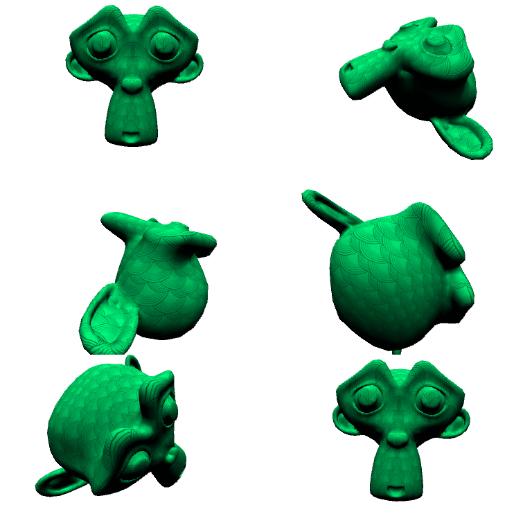

A major difference between vectors and normals is the way a normal’s scale is calculated when the surface it represents change scale. Furthermore, normals cannot be added to a spatial coordinate or created from subtracting two coordinates.
We prioritize those vector functions upon which future operations depend. More can be implemented by looking at the PVector class; there are also functions, such as reflect and scalar projection (see Shiffman’s video to the left), not contained in PVector but nice to have.
Dimension
The next Transformable is a nonuniform scalar, which has width, height and depth. Below are a few highlights.
The best way to understand this class is to think through why a vector is a bad way to represent dimension. First, although minor, are variable names: x, y and z do not describe this class’s fields. Second, while a vector resets to (0, 0, 0), a dimension resets to (1, 1, 1). Third are key differences in how addition, subtraction, multiplication and division work. Adding a single float value to a dimension means adding a uniform scalar to a nonuniform scalar; a single float can’t be added to a vector. As we saw earlier when decomposing a matrix, vectors have scalar, dot and cross product operations; they cannot be multiplied by three separate floats.
Rotation
Since quaternions were introduced in another tutorial, we’ll only touch on new methods.
The forward, right and up functions allow us to access and display the orthonormal basis of a shape. These are the unscaled i, j, and k columns of a matrix. Quaternion multiplication provides the analog to nesting one call of pushMatrix inside another. If we recall that a quaternion can be represented either as four numbers or as an imaginary vector and a real number,

we can express quaternion multiplication as

Division, which depends on the invert function, is a rough analog to popMatrix. Like 2D complex numbers, a quaternion’s inverse depends on its conjugate,

which is the negation of its x, y, and z components. The conjugate is then divided by the quaternion’s magnitude-squared.

Returning to our wishlist, it’s not clear that rotateX and company are functions to rotate geometry by an angle around the x-axis. Furthermore, this could be another case where functionality should remain unimplemented. Rotation by x, y and z encourages sequential Euler angle rotations, rotation.rotateY(theta).rotateZ(theta);, a habit we want to get away from.
Brittle Class Hierarchies

Fans of the meta will notice that the hierarchical tree we’re developing describes the code’s design itself.
In the diagram, left, interfaces are color-coded in red; abstract classes, in green; and classes we instantiate into objects, in blue. Organizing these classes is a negotiation between what an object is, what it does and what kind of data it has. The negotiation is muddied by the fact that any action a class does can be coded as a method or as a ‘behavior’ object the class has.
Any satisfaction to be gained in arranging classes neatly is flustered by the brittleness of hierarchies. Such diagrams offer the impression that coding can be and is always planned in advance. That frequently conflicts with creative coding’s emphasis on prototyping, iteration and exploration. Once we add new features, this illusion of order collapses.
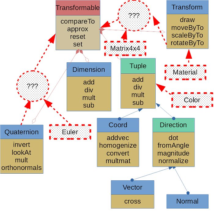
Eventually, an introduced class will find multiple candidates to be its parent; or will for the sake of belonging find the least unlikely parent to extend. A child class will inherit from its parent a behavior that undermines its identity, but which it cannot conceal. A parent will hold onto information it doesn’t need for the sake of its children. Two classes which should belong together conceptually will have so few data types in common that all we can do is add a marker interface for them. The closer to the root these problems occur, the bigger the hassle in revising code.
Having raised the issue of inheritance hierarchies, resolving it in Java would take us far afield of the subject at hand. We move on to the transform class, trusting that those interested in resolving the above will find a design pattern best suited to the job.
Transform Classes
We may animate not only a coordinate in sketch space, but also a texture coordinate that maps an image onto a model’s geometry. For that reason, we split a material from a transform, and make a abstract TransformSource parent class. Convenience is the primary consideration for this class: a majority of functions are wrappers that provide intuitive function names.
These wrappers allow us to meet our criteria, specifying when a function transforms by a value and to a value. Since we cannot avoid PMatrix objects entirely, we provide conversions similar to those earlier, decomposing into quaternions instead of Euler angles.
For the Transform class, we extend the above and add the following
For diagnostic purposes, we draw red, green and blue lines showing the transform’s axes. The parent field allows transforms to nest one within the other, replicating the nested calls to pushMatrix. This complicates our ability to find the position, rotation and scale of the transform relative to the sketch, not its parent.
An alternative would be to create a tree or node class which has a Transform object. For that approach, Stack Overflow discussions are here and here.
Applying Transformations
To apply a transformation to a point, we add methods to the Tuple class. Convention sometimes call these applyTo and reverse which object owns them. For example, a quaternion would have the function applyTo(Tuple t).
As seen above, translation is influenced by rotation and scale. So while rotation has a direct correlation with multiplication by a quaternion, and scaling with multiplication by a dimension, translation is the addition of two tuples after multiplication by rotation and scale.
Example: Spirograph

With the above in place, we can try for a digital Spirograph, dressing it up with translucent backgrounds and blend modes.
Adding a translucent background panel to a sketch is a common technique among creative coders to give animations a contrail or, depending on the blend mode, a diaphanous look. In 2D, fill(0x7f000000); rect(0, 0, width, height); will suffice; 3D is less intuitive, given the potential of a moving camera.
Because a point could pass behind the background, we disable all activity related to testing depth. If we animate the camera, we first cache its default orientation in a PMatrix3D, then pass that into the function. Later, we’ll introduce an alternative that uses rendering techniques better suited to 3D geometry.
A Custom Mesh
In an earlier tutorial on 3D modeling we introduced .obj files, which can be imported into Processing via loadShape. By disconnecting from matrix transformations, we’ve lost the convenience of this function and the object it returns, a PShape. In the following section, we develop our own.
WaveFront .obj File Format
To understand what we’ve lost and how it can be regained, let’s review the .obj file format. The example below describes a cube.
Information is preceded by a key: the object’s name begins with o; a vertex, with v; a texture coordinate, with vt; a normal, with vn. Data for the face, preceded by f, are most in need of explanation. Simulating the cube’s front face will help to understand.
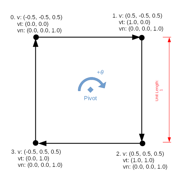
The pivot point around which all vertices rotate is (0, 0, 0), so we start winding at the top-left corner, then proceed clockwise to the top-right corner. (Instead of using 0.5, we can dub the edge A (-1, -1, 1), B (1, -1, 1), giving it a length of 2.) Because the front face of this cube shares each of its four edges with four other faces, and because each edge shares its vertices with other edges in this face and in other faces, we have to store data without duplication and access it out of sequence.
If we think of the data in the v, vt and vn sections as arrays (assuming that they have been calculated and included) the face section contains indices to these arrays, separated by a forward slash /.
Mesh Class
With this in mind, we can parallel the .obj format in working memory with
We need to be explicit about passing by reference versus passing by value, a silent distinction in Java. Whenever we pass an object into a function, we are passing a reference to its memory address, not an independent value which can be changed without also changing the original. In order to leave the original object intact, we copy the primitive floats that it contains.
We’d like load mesh data from an .obj file once, then share this ‘template’ among many entities that are transformed independently of one another. Also, we want to manipulate a mesh procedurally then export the changes as an .obj file. An entity’s transformation would have no effect; we’d need to copy the mesh data, then manipulate the mesh and not the entity. (For those familiar with Blender or modeling software, this is the distinction between Object and Edit mode.)
Acquiring Faces and Vertices
When accessing and mutating that data, for convenience we’ll want not the indices, but the data pointed to by those indices. To do this, we create a vertex and face class:
and
To retrieve them from the mesh, we return to the Mesh class to include
These provide a workaround to limitations of PShape, whose getChild, getVertex, getNormal, getTextureU and getTextureV functions are messy. Moreover, this workaround follows a pattern for augmenting Processing to handle intermediate projects: what we need is already at work behind the scenes; we expose it while subdividing tasks for a finer granularity.
Even so, the ability to edit a mesh exposed by these classes is fairly basic. Edges, for example, are nowhere represented; the ability to find the neighboring faces of a face is absent. Greater nuance may be found in the half-edge data structure, for which a library, HE_Mesh, is available.
Importing An Obj File
Given the linear format of an .obj file, loading and saving one is easier to do than we might first imagine. We’ve simplified Processing’s import function in that we assume a file will always include texture coordinates and normals. A robust function would handle scenarios in which the information is absent by, for example, supplying default values.
At the end of our import function, we expect a fixed number of coordinates, faces, etc. However, at the beginning, we don’t know how many an .obj file will contain. For that reason, we create lists which, unlike arrays, can expand when new information needs to be added. We convert these to fixed-size arrays with toArray at the function’s end.
This task falls under the heading of tokenization. Processing’s loadStrings function has already taken care of splitting up the selected file by line-break into an array of Strings. On each line, information is split up by whitespace, so split("\\s+"); separates tokens by that. The first token determines which category we go to in a large if-else block while the remaining tokens are parsed as either floats or, in the case of faces, ints. Faces is a special case in that it is broken into sub-groups by /.
Exporting An Obj File
Writing a file is easier than importing one. A library to export .obj files, courtesy Nervous System, is also available. The one trick that may be new is how to avoid concatenation of Strings with the + operator. Two tools to aide with that are the String.format function and the StringBuilder object.
We leave aside the matter of importing materials, since a material’s capability varies greatly across graphics engines, and depends on underlying shaders.
Material Class Definition
Instead, materials are created through a Material class.
As a reminder, emissive color is given off without any lighting in the sketch. Ambient color responds to atmospheric lighting with no discernible direction or source. Specular color defines the glint that reacts to directed light sources. Shininess is the gloss of a material. This abstract super class can then be extended to handle a texture.
Texture mode dictates how Processing interprets the texture coordinates supplied to vertex. Processing uses the pixel size of the source image by default, not coordinates in the range 0 .. 1. Using NORMAL allows source textures of varying dimension to be mapped consistently onto a shape. Texture wrap dictates what happens when a texture coordinate exceeds the range set by texture mode; REPEAT allows a texture to look like a wallpaper.
Drawing An Entity
As mentioned earlier, we must distinguish between the animation of underlying mesh and of an object in space which draws that data. For this reason, we create an Entity class.
The v, vt, vn and wr variables ensure that no transformation becomes permanent. For now we, are simplifying our Entity class; a more developed approach would be to create an Entity-component system. To see this in action
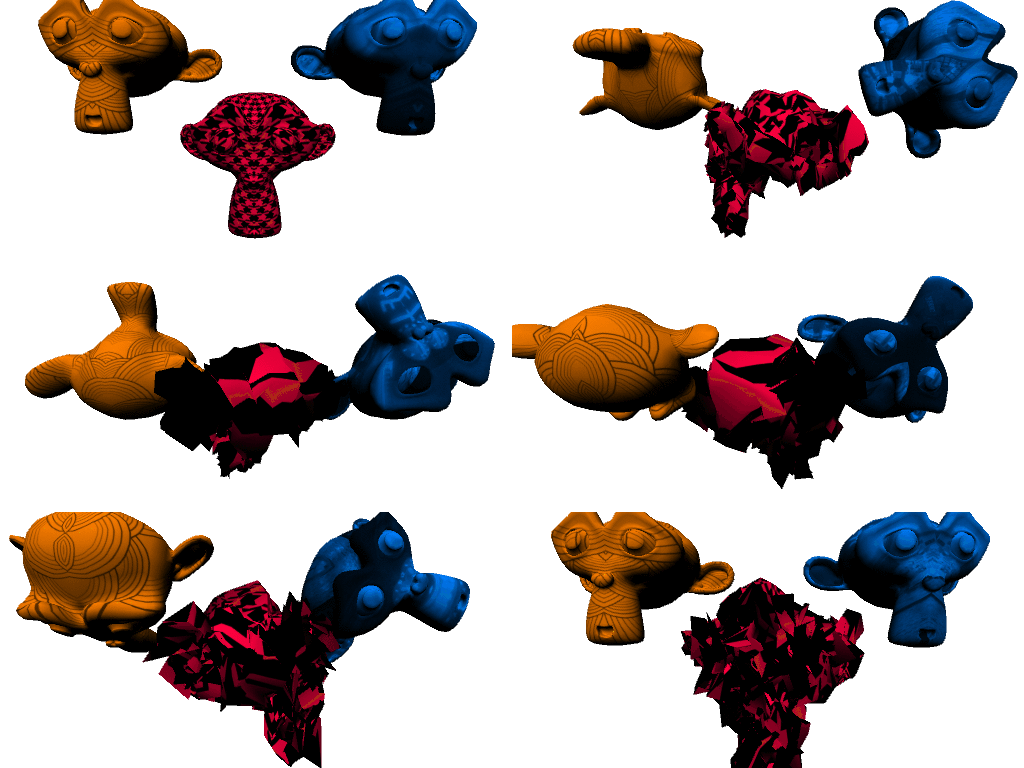
we create three entities, each of which has an animated material and transform. The magenta figure, bottom-center, retains a copy of the mesh data, which it animates in draw. To see what does and does not carry across upon export, and how the qualities which are not exported can be recreated, we import it into Blender and into Unity.


Neither the scaling of the UV coordinates by the material nor the rotation by the transform are retained, but the addition of random values to the underlying geometry are. Both Unity and Blender provide the option to recalculate the normals according to their own world coordinates.
Easing
A major reason to use quaternion-based transforms is to better facilitate easing (or tweening) between positions, rotations and scales. Because we don’t know in advance which kind of tweening we’d like to use (lerp, ease-in, ease-out, etc.) we externalize this behavior. First, we code an umbrella class to cover all the variety
The passing of behaviors as objects back and forth is not as natural to Java as it is to JavaScript. The library java.util.function offers some classes, and we can also specify a @FunctionalInterface with an annotation if we need more. This parent class handles the logic for easing between a start and stop keyframe or for easing between an array. The logic specific to each kind of easing, applyUnclamped, is left to subclasses to define. As an example, to ease between tuples, we use
referencing Ana Tudor’s “Emulating CSS Timing Functions with JavaScript” for ease-in and ease-out. The easing of dimensions and quaternions follow a similar pattern, so we won’t cover them here. We can then lump these together into a transform easing behavior.
Were we to make any provision for a Color class, we could decide upon easing between colors in RGB and HSB, then incorporate that into Material easing classes. For those interested in such a possibility, a previous tutorial on color gradients may provide reference. Put into effect, these look like

Because frame rate is now a concern, we use a simpler diamond geometry. Instead of creating a rectangle shape with translucent fill, we use createGraphics to create a second renderer. This can have a transparent background.
In draw, we update the second renderer, then blit it onto the main sketch renderer with image. This has the benefit of rendering at one scale, then either up- or downscaling to the display. We have greater control over how we capture stills depending on which renderer saves the image. A disadvantage is that residue may appear on the edges of geometry when a translucent background is used on the secondary renderer.
Conclusion
When reaching the end of a first iteration, it is worth returning to our wishlist to see if we’ve met any of our goals. Additionally, we can ask what artistic potential is opened by the coding we’ve done. One possibility is to look at examples of the Twelve Principles of Animation and set ourselves the challenge of recreating them. Another would be to explore basic skeletal and pendular movements enabled by nested transformations.
