3D Models In Processing

To sharpen our skills with lighting, color and materials in Processing’s 3D renderer, it’s helpful to have a model more complex than a geometric primitive. The Processing core handles .obj files, so we convert any resource to that file extension before we can work with it. In the demo to follow, we bring in sculpture available from Scan The World. To do so, we would benefit by strengthening our pipeline between Processing and modeling software. We have chosen to use Blender but other possibilities, such as Autodesk Maya, are out there.

Blender has the advantage of being powerful, free and flexible; the downside of those virtues is that learning how to use it requires patience for those accustomed to standardized interfaces in Adobe Creative Cloud and/or Microsoft Office. Since there are many excellent tutorials dedicated to learning Blender, we will be as brief as possible, establishing the essentials. We use Blender version 2.78 for the screen captures below.

Getting Started With Blender

Upon installing and running Blender, our first step is to ensure we can import and export the file formats we need. In our case, we need to import .stl (stereolithography) files from the aforementioned website and to export .obj files. To accomplish this, we go to User Preferences, then click on the Add-Ons tab.

This serves the same function in Blender that the Contribution Manager (under Tools > Add Tool…) does in Processing: we expand the capacity of the core software with both official and community created add-ons.

We can browse for add-ons by category, listed on the left, or search for keywords. If we search for “OBJ”, we find the add-on Import/Export: Wavefront OBJ Format. The white twirly on the left of the entry allows us to view information about the add-on. Ticking the check-box will enable it. Some add-ons may need to be downloaded. We do the same for Import/Export: STL Files.

Turning now to the 3D viewport, we see a scene with a Camera, Cube and Lamp. We also see these listed in the Outliner panel. If we press the A key to toggle select/deselect all items in the scene, then the Delete key, we can remove these elements.

Next, we import our model through the File menu.

After navigating through the file browser and clicking Import STL, we should see the model we want in the editor… Though, depending on how well it was prepared, we may need to zoom using the mouse’s scroll wheel or to pan by holding Shift with the scroll wheel. The model may not be centered on the origin, which would make positioning it awkward in Processing. To fix this we open the Object menu on the bottom tool-bar, then go to Transform > Geometry to Origin. If the tool-bar isn’t visible, click on the + in the bottom-right of the 3D view. If the tool bar is visible, but the Object menu is not, make sure that Blender is in Object Mode from the drop down menu.

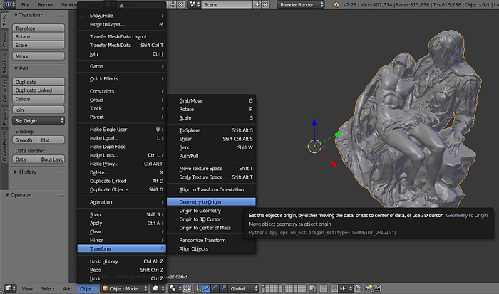
For this exercise, we use Michelangelo’s Pieta in St. Peter’s Basilica.

Processing, Three.js, Unity and other engines render real-time, dynamic, interactive graphics; we cannot always wait for a frame to render. Externally sourced models may have been created to represent real-world geometry with high fidelity, or for use in high-resolution non-interactive renders. Often, we reduce vertices in our models so as to not drag down the frame rate. To do this, we go to the Properties panel, typically on the right, then click on the wrench icon at the top of the panel. In the Add Modifier drop-down menu, we then select Decimate.

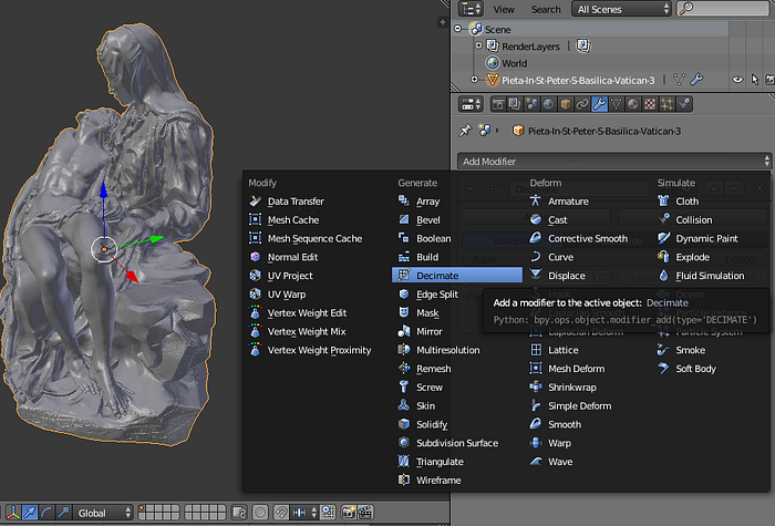
The Decimate information will indicate how many faces the model contains. In the illustration of the Pieta below, we begin with 815,738, which we reduce to 16,314. We accomplish this by selecting the desired Ratio by which we want to decimate our faces, 0.02, then click Apply. Alternatively, we could switch from Object Mode to Edit Mode then go to the menu Mesh > Clean Up > Decimate Geometry.

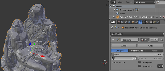
If we wish to smooth the low-poly look, we select Smooth Shading instead of Flat Shading in the panel on the left, under the Tools tab.

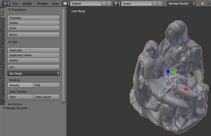
Up on the y-axis and forward on the z-axis are not always standardized across 3D software packages. While in Blender, the origin and a RGB color-coded indicator keeps us oriented. However, for some models, the matter is further confused by stage forward vs. camera forward, stage left vs. camera left, etc. (We may think of scenery facing the camera as facing forward, while an avatar walks forward with his or her back to the camera.) In Processing, a positive or increasing y value proceeds downward while a negative or decreasing value proceeds upward. A positive or increasing z value proceeds toward the view-port while a negative z value recedes toward the horizon.

We have a few options in dealing with this. To rotate our model, we can go to the Properties panel, click on the gold cube to select the Object tool, then rotate as needed.

We could also mirror and/or scale, since Blender units are not the same as Processing’s, or wait until we are ready to export.

File Export and Format

By going to File > Export, we pull up the directory browser. In the lower left corner there are many settings, among them drop-downs for Up, Forward, as well as a Scale multiplier.

We next click on Export OBJ in the upper right corner. By default Blender writes not only an .obj file, but a .mtl file as well. We may want to take a moment to open these two files in a text editor to better understand them. A minimal .mtl file looks like so

A .mtl file is a library, meaning it may contain multiple materials. The # indicates a comment just as // would in Processing; Blender generates a comment to inform us of the number of materials to follow. The newmtl keyword, followed by a name, designates the start of a new material. Ns specifies material’s shininess. Ka specifies the ambient color, followed by the Red, Green and Blue channels in a range from 0 to 1. Kd specifies diffuse color. Specular color is defined by Ks. These three qualities will be explained in further detail below, when we change them within Processing. Transparency, also called dissolve, is specified by d; changing this value produces no effect in Processing. Lastly, the illum keyword followed by the number specifies the manner lighting is simulated. Further explanation for this and other elements of the file specification can be found here.

The .obj file is too large to reproduce in total here, but an abridged version is arranged like so

mtllib specifies which .mtl file to look up, and, further down, usemtl names which material defined in that library to use. o prefixes the object’s name. Lines beginning with v issue 3D coordinates for vertices; vn, normals, vectors perpendicular to a surface which indicate the direction it should face; vt, absent in the above, indicate how a 2D texture is mapped onto the geometry’s 3D form. The s off states that flat shading, rather than smooth, is used. Lines beginning with f represent the faces formed by the model.

Because of the dependency in the .obj file, were we to add it to a Processing sketch (go to the tool bar, select Sketch > Add File or drag and drop the files onto the sketch window) without also adding the .mtl file, we’d see in the console a message such as The file “sketchPath\data\pieta.mtl” is missing or inaccessible, make sure the URL is valid or that the file has been added to your sketch and is readable. If we want to set the material properties entirely within Processing, we could delete the .mtl file and in the .obj file delete the mtllib and usemtl lines. With that cursory look at these files, we’re ready to import.

Importing

We bring our model into Processing with the following

Instead of translating the model to the middle of the screen, we move our perspective camera to look at the origin. Default lighting includes an ambient light and a directional light, with the latter pointed forward. There is no specular lighting, which means the edges of the model will not glint. The backside of the model will be lit by only the ambient light.

It’s worth breaking the default lighting down into its constituent elements so that we can better control and observe how lights interact with the material as we make changes.

The first three parameters of both ambient and directional light refer to the lights’ color, a neutral mid-gray. Ambient light is a refracted light which permeates the atmosphere of our sketch. Directional light is more like the sun’s rays through a window; what counts is the direction the rays are pointed. We will keep these neutral for now and instead adjust the shadow, diffuse and highlight colors of our model.

Setting Material Properties

If we add pieta.setFill(0xffff007f); to setup, we change our diffuse color to a magenta. For this and other material setters of PShape that follow, the argument accepted is a color; if we wanted our code to be more intuitive, we could use pieta.setFill(color(255, 0, 127, 255));.

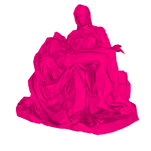
Throwing pieta.setAmbient(0xff7f7f00); into the mix adds a mustard tint to our model.

If we turn off the directional light by commenting it out, we see this dark-yellow exclusively, as it responds to the ambient light.

The specular quality of the model’s material responds to directed light rather than ambient light; to illustrate it, we comment out the ambient light, comment the directional light back in, and change the latter’s direction from forward to downward directionalLight(128, 128, 128, 0, 1, 0);. We also crank up the specularity for all lights in our scene lightSpecular(128, 128, 128);. Finally, on the model itself, the specular reflection is set to a blue leftPieta.setSpecular(0xff0000ff);.

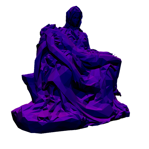
Turn everything back on and we see the not altogether pleasing but at least illustrative

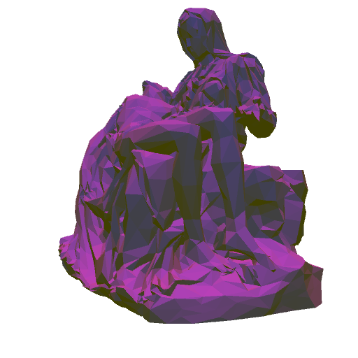
Not pictured above, we can also set the emissive quality of our model, meaning it will emit light of that color independently of any light in the scene pieta.setEmissive(0xffff0000);. This alone is not sufficient to make a model appear as though it were itself a source of light; no light will be thrown on to nearby objects, nor will there be a halo. It can, however, give an object an uncanny aura in an otherwise dark sketch.

Dynamic Lighting

Now that we’ve tested our material properties, we can play with lighting. In addition to ambient and directional light, we also have point light — undirected, radiating outward in a sphere, and positioned in space — and a spot light — spatially positioned, directed, and extended as a cone. Whenever spatial position can be specified, it can also be animated. To demonstrate, in the following

we have three spotlights. The first points a teal light to the East and slides up and down the left edge of the sketch. The second points a green light down and slides left and right across the top edge of the sketch. The third simulates a flash light, as it is held at the camera’s position, faces forward and then points toward the mouse’s location normalized to a range 0 .. 1. Its concentration oscillates between 12 and 100.

A second example makes use of point lights and emissive materials. The code below

provides the following results

lightFalloff influences all lights, but for sketches heavy on point lighting it is key to adjust how far light reaches so we can fine-tune how point lights influence their neighbors. One last observation is that Processing limits the number of lights we can use in our scene to 8. This bears mentioning for anyone intending to create a circle of candles, stars, etc.

UV-Mapping

Our .obj file currently contains no information for how to map a 2D image onto 3D geometry. This information is commonly set down with uv coordinates, and, when included, is prefixed in the file by vt. Without it, setting a texture on a model in Processing would only produce a solid color. We return to Blender to introduce uv-mapping.

If we look on the bottom of our editor, we should see another window which we can expand vertically by dragging with the mouse. This is usually set to the Timeline view (represented by a clock). If we click on the drop-down menu, we can change to UV/Image Editor.

Now that we have different options, we can open an image to serve as our texture. If we don’t have one ready to hand, we can create a new image by clicking on the + and choosing UV Grid from the Generated Type drop-down.

Were we proper texture artists, we’d select edges of our model in Edit Mode, mark seams, manually unwrap and place our UV coordinates on a map, and then paint onto our model in 3D, save a template and work in an external graphics environment, etc. For those interested in the manual approach, this video tutorial is worthwhile. For the time-being we will take advantage of Blender’s automated unwrapping functions. In preparation, while in Object Mode we select View > Front. (We may also want to temporarily rotate the model to face up in Blender.)

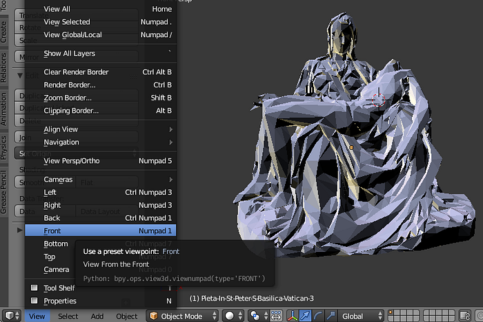
Switching to Edit Mode, we select all our vertices by pressing A, then go to the Shading/UVs tab in the left panel and select Project from View (Bounds) from the drop-down. A flattened mesh will appear in our UV/Image Editor panel. By clicking on the UVs menu we can mirror, translate, rotate and scale this mesh if we so desire. We can also select Reset and try out other projections.

Depending on the manner of projection, more or fewer pixels may be stretched over a face on the model. If we want to preview how this will look before we export, we should add a light source. Switching back to Object Mode, we go to Add > Lamp > Sun.

We now add our image to the material on the model. Assuming a material and texture already exist, in the Properties panel on the right, we click on the red and white checkerboard to switch to Texture information. Under the Image section we then select the image file of our choice.

We preview our map and texture by clicking on the drop-down in the view-port with the little white ball and selecting Rendered. If we wish to change any material qualities, we can click on the checkered orange and black circle in the panel to the right.

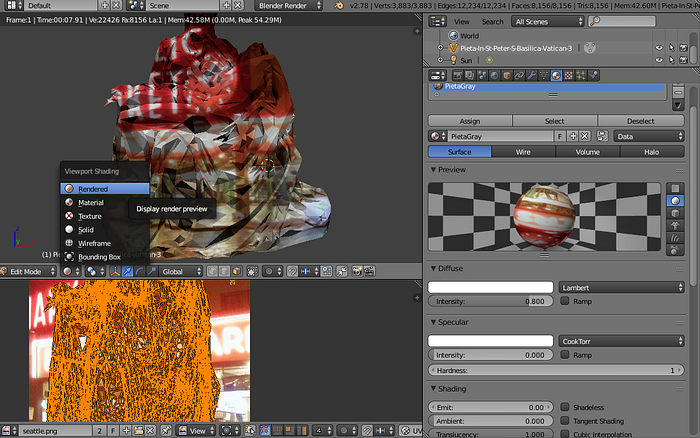
Upon exporting and opening this in Processing with our initial code base, we add a line pieta.setTextureMode(NORMAL);. Blender writes the uv coordinates for our texture map in a range of 0 .. 1, while Processing accepts pixel coordinates by default. We see

If a message appears in the console indicating that the image file could not be found, we can open the .mtl file to change the file path prefixed by map_Kd from an absolute to a relative path, in this case seattle.png. This assumes, of course, that our image is already in our sketch’s data folder.

Setting A New Image

We are not limited to PImage files; children of PGraphics are fair game. Suppose we wanted to project a webcam capture onto this model. If we go the Tools menu and select Add Tool…, we open the Contribution Manager. By clicking on the Libraries tab and searching for “Video”, we can download and install the official video library.

Next, we can make some adjustments to our earlier code:

We don’t have to work with the webcam feed or video directly, either. As discussed in another tutorial, we can loop through all the pixels of an image and alter their color according to a set of rules. Working from the above, we develop our code into

We create a second PImage for a texture. In draw, we loop through every pixel of the webcam image and evaluate the brightness of the pixel at position (x, y). Although an image is two-dimensional, the array of pixels is one-dimensional, hence the incrementing of i in the inner for-loop. If the pixel brightness is greater than the threshold, then we replace the original color with one of our choosing for the highlight, and so on to mid-tone and shadow. We update the pixels of the txtr to reflect these changes and display our scene as usual.

Dynamic Geometry

To better understand the capabilities of a PShape, it’s better to use the Javadocs than the reference. As a matter of convenience, however, the best bet is to open File > Preferences… and tick the Code completion with Ctrl-space box so autocomplete lists available behaviors and properties as we type.

One behavior in particular merits exploration. Suppose we want to change the vertices of our model in the draw loop. myShape.getVertexCount(); seems like it would return the max number of vertices, allowing us to loop through them, acquiring each vertex with myShape.getVertex(i); and updating it with myShape.setVertex(i, x, y, z);. However the vertex count returned is 0. Why? A quirk of how .obj files are interpreted is that each face is a child shape of the parent shape. As explained by a contributor to Processing here:

the OBJ parser creates a separate child shape for each face, the main reason begin [sic] to allow faces to have separate materials (because Processing only supports single texturing of shapes), and also because each face is not necessarily of the same kind (triangle, quad, general poly).

Updating vertices and then displaying the face on a model of any considerable detail is unlikely to be performant with the approach above. Multiply 1000 or more children by 3-4 vertices, and the calculations add up. To demonstrate how we might manipulate, if not the vertices, then the faces, we use a simpler model: Suzanne the monkey head from Blender.

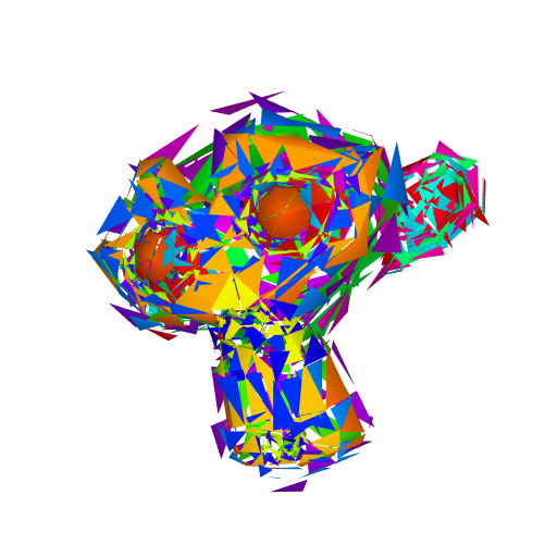
We color-code each child by hue in setup, then translate randomly in draw. Another possibility for acquiring vertices suggested by Dan Shiffman in the aforementioned thread is to use getTessellation();. Expanding on Shiffman’s work, we demo the following; this time, with a bust of Julius Caesar.

We use two PVector arrays, one to cache the vertices which represent the model acquired from the tessellation, another to represent “exploded” vertices. The points displayed in the sketch oscillate between these two positions. For illustration, our exploded vertices form a curlicue, but more imaginative applications are possible: these particles could form a plexus, flock or circulate through a particle system.

Putting It All Together

Now that we know how loadShape anticipates a more complex use-case than we need, that getTessellation allows us to simplify our approach, and that we can transition between a generated form and a premeditated form, we can ask the following: could we morph one model into another if they had the same number of faces and vertices?

The earlier mentioned problem of there being an irregular number of vertices per face can be alleviated by ensuring in Blender that both models use tris (3 vertices per face) by switching to Edit Mode, then selecting the menu Mesh > Faces > Triangulate Faces or by applying the Triangulate modifier. The Decimate modifier used earlier will allow us to match the number of faces of two models.

Remembering the data stored in an .obj file, we can now think about how to store those for both our models. A Pshape stores faces from getTessellation; PVector arrays can store vertices, normals and uvs. For the example to follow, we’ll add in a model of the bust of Nefertiti.

Since our transition between Nefertiti and Caesar is governed by lerp, we can control the state of disintegration by remapping our mouse position to 0 .. 1. We’ve used the webcam library to animate our texture by frame, but we can also animate the texture uvs. Updating a uv offset or scale allows us to create repeating patterns or simulate an infinite flow over the geometry’s surface; if we opt for such an effect, we add textureWrap(REPEAT); , as the default is to clamp the texture.

There is one stray material property, shininess, which we did not encounter above. It might be described as how dramatic the change between shadows, mid-tones and highlight are. Materials with low shine appear muted, dull; high shine materials are said to sparkle or have gloss.

Conclusion

Hopefully, this article has shown the importance of working between development environments to create a workflow, not just a piece. As we come to understand the concepts behind 3D geometry, many of the same effects can be created across and between applications; in some cases a text editor is all we need to change how a model shines in the light. Were we to switch from Processing and Blender to other software, our skills would still apply.

As always, learning technique is only the beginning. With some basics covered, strengthening aesthetic sense would be a next step, for example, how a face might be lit to create a dramatic mood or how different material qualities make an object stand out to a viewer. On this, below is a fun video in closing.